On this page
Recursive Language Models are having a moment. The original paper by Zhang, Kraska, and Khattab showed that instead of cramming documents into ever-longer context windows, you can let an LLM programmatically explore its data, calling tools, delegating sub-tasks, and iterating until it finds what it needs. DSPy’s experimental dspy.RLM module brought the pattern to a broader audience. Viral posts about auditing codebases for 87 cents caught everyone’s attention (worth noting: even that experiment frames itself as a demo, not a replacement for a real security audit, and reruns catch different issues). Prime Intellect called RLMs “the paradigm of 2026.”
We agree. We’ve been running RLM-style workflows in production using ZenML’s dynamic pipelines, and we wanted to share what we learned about making them observable, debuggable, and cost-controlled.
We’re not here to replace DSPy or any other framework. We’re here to show what happens when you wrap the RLM pattern in proper orchestration.
What Are RLMs? A Quick Primer
If you’ve heard the buzz but haven’t read the paper, here’s the short version.
The Problem: Context Rot
When you stuff massive documents into an LLM’s context window, performance degrades. Even models with 200K+ token windows lose accuracy as the prompt grows. This is a measured phenomenon, not just vibes.
Long context windows do not guarantee long-context competence. Controlled studies show models can be sensitive to where the relevant information sits (“lost in the middle”), and that popular “needle in a haystack” tests can overstate real performance because they reward lexical matching. When lexical cues disappear, performance drops sharply with longer inputs, even for models marketed as long-context. Chroma’s “context rot” report shows that even with simple, controlled tasks, performance degrades with increased input length, and NIAH is not representative of real workloads.
A helpful way to think about why long context fails is: how much work must the model do as the prompt grows? Some tasks are essentially constant-complexity (find one needle). But many real problems scale with the amount of information. You need to scan most items (linear), or compare many pairs (quadratic). The RLM paper uses this exact ladder in its evaluation, and it explains why models can look great on needle tests yet collapse on aggregation-heavy tasks.
The RLM Solution
Instead of feeding everything into one prompt, RLMs treat the context as a variable the model can programmatically explore:
- Store the context externally (in a REPL environment, a database, a file)
- The LLM writes code or selects tools to peek at, search, slice, and process the data
- The LLM can recursively call itself (or cheaper models) on sub-chunks
- A "root LM" orchestrates the process and assembles the final answer
Think of it this way: instead of reading a 10,000-page archive cover-to-cover, you sit at a desk with the archive in filing cabinets. You write a research plan, pull specific folders, delegate sections to research assistants. You never try to hold everything in your head at once.
Key Results from the Paper
The numbers are striking:
- RLMs can handle inputs up to two orders of magnitude beyond model context windows
- RLM-Qwen3-8B (a Qwen3-8B model fine-tuned to run inside the RLM scaffold) improves median performance by 28.3% versus an untuned Qwen3-8B running in the same RLM scaffold, across the paper’s four long-context evaluation tasks.
- On three tasks where the paper reports a meaningful direct GPT-5 baseline (CodeQA, OOLONG, OOLONG-Pairs), RLM-Qwen3-8B closes much of the quality gap to a direct GPT-5 call. On BrowseComp+ (1K documents), the full input does not fit in a direct prompt baseline, but the RLM scaffold can still operate.
- Cost is comparable or lower than direct LLM calls at the median (more on the variance later)
- It's primarily an inference strategy, not a training method: it works as a wrapper around existing LLMs (though a small amount of training can improve scaffold-use)
The paper’s evaluation includes tasks where base models cannot even fit the input. BrowseComp+ at 1K documents is in the multi-million token range. RLM variants can still operate.
How RLMs Differ from RAG
People sometimes confuse these. They’re quite different:
- RAG retrieves chunks via embedding similarity. It's essentially a search engine: your query gets turned into a vector, and the system finds the nearest chunks.
- RLMs programmatically explore data. The model decides what to look at, what to search for, and what to delegate. It's a research assistant with a filing system, not a keyword search.
RAG retrieves. RLMs investigate.
RLMs are also part of a broader pattern: systems that treat “what’s in context” as a first-class design problem. Recent work on context folding and proactive context management explores different approaches. RLMs push this further by letting the model programmatically explore externalized context instead of compressing it into a single prompt.
The Production Gap
So the RLM pattern is powerful. dspy.RLM is excellent for prototyping and research. The trajectory output is fascinating: you can see what the model did, step by step. Budget knobs like max_iterations and max_llm_calls give you cost control per call.
But when you start running RLMs in production, new questions come up:
- "I ran this on 500 documents. 3 chunks failed. Which ones? Why?"
- "How much did each chunk cost? Where are my dollars going?"
- "Can I cache the results so I don't re-process unchanged chunks?"
- "This works on my laptop. How do I run it on Kubernetes with 50 chunks in parallel?"
- "My teammate wants to understand what the model did on chunk 17. Where do I point them?"
There’s also a less obvious concern: variance. RLM-style loops can have a heavy tail. The RLM paper reports cases where the median RLM run is cheaper than the median base-model query, but some RLM outliers become significantly more expensive, driven by long, variable-length trajectories. This is exactly the kind of tail risk that feels fine in a notebook and becomes painful at scale, unless you have per-chunk cost attribution, caps, and retries.
These are orchestration problems. DSPy is a framework for building LLM programs. ZenML is a framework for running them in production. They’re complementary layers.
ZenML Dynamic Pipelines as the RLM Runtime
The Structural Parallel
The RLM pattern and ZenML’s dynamic pipelines have the same shape:
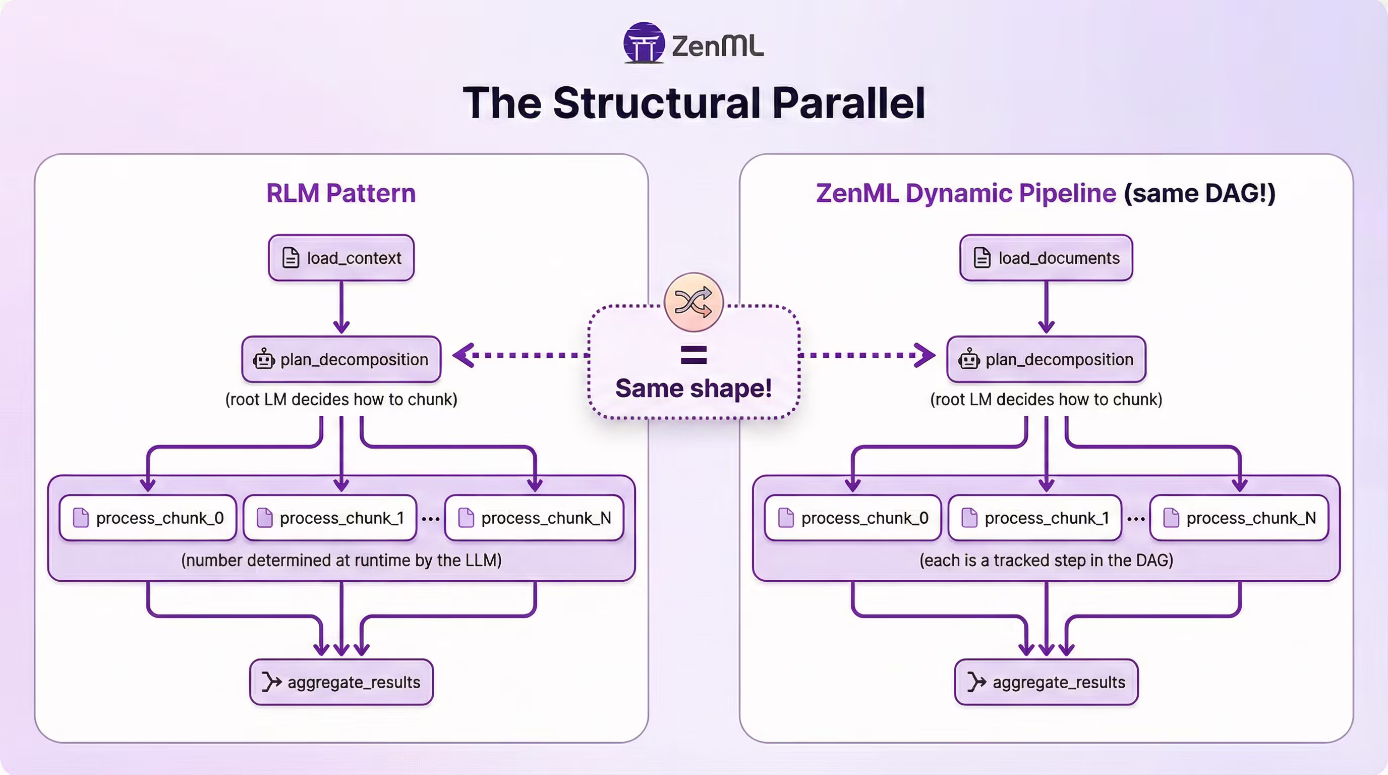
The number of process_chunk steps is decided at runtime based on the query and corpus. ZenML auto-names repeated invocations (process_chunk, process_chunk_2, etc.).
The Key Mechanism: .load() vs .chunk()
Here’s the core of the dynamic fan-out, straight from the pipeline code:
@pipeline(dynamic=True, enable_cache=True)
def rlm_analysis_pipeline(
    source_path: str = "data/sample_emails.json",
    query: str = "What financial irregularities or concerns are discussed?",
    max_chunks: int = 4,
    max_iterations: int = 6,
):
    # Clamp budgets to prevent resource exhaustion
    max_chunks = min(max(max_chunks, 1), 10)
    max_iterations = min(max(max_iterations, 2), 12)

    # Step 1: Load and summarize the corpus
    documents, doc_summary = load_documents(source_path=source_path)

    # Step 2: Decompose into chunk specs
    chunk_specs = plan_decomposition(
        doc_summary=doc_summary, query=query, max_chunks=max_chunks
    )

    # Step 3: Dynamic fan-out — one process_chunk step per chunk
    process_step = process_chunk.with_options(
        parameters={"query": query, "max_iterations": max_iterations}
    )

    chunk_specs_data = chunk_specs.load()  # Materialize for control flow
    chunk_results, chunk_trajectories = [], []
    for idx in range(len(chunk_specs_data)):
        result, trajectory = process_step(
            documents=documents,
            chunk_spec=chunk_specs.chunk(index=idx),  # DAG edge per chunk
        )
        chunk_results.append(result)
        chunk_trajectories.append(trajectory)

    # Step 4: Synthesize all chunk findings
    return aggregate_results(chunk_results, chunk_trajectories, query)
Two ZenML-specific APIs are doing the heavy lifting here, and they’re easy to confuse:
.load()means "bring this data into Python so I can make a decision." Here, we loadchunk_specsto learn how many chunks the LLM created, so we know how many times to loop. It's synchronous..chunk(index=idx)means "create a DAG edge to this specific element." Eachchunk_specgets passed to its ownprocess_chunkstep without materializing the entire list. This is what creates the dynamic fan-out in the DAG.
What You Get for Free
Here’s the practical comparison:
| Capability | Notebook/Script | ZenML Dynamic Pipeline |
|---|---|---|
| Recursive sub-calls | Yes (in-process) | Yes (each is a visible step) |
| Per-chunk observability | Manual logging | Built-in: metadata, artifacts, logs |
| Cost tracking per chunk | DIY | log_metadata per step |
| Caching unchanged chunks | No | Artifact caching |
| Retries on failed chunks | DIY | Step-level retries |
| Visual DAG | No | Dashboard shows runtime shape |
| Run on K8s/Vertex/SageMaker | Manual infra | Stack abstraction |
Inside the RLM-inspired Loop
Our production example is RLM-inspired rather than a line-by-line reproduction of the paper’s REPL-based Algorithm 1. Instead of letting the model write arbitrary Python in a REPL, we constrain it to a small set of typed, deterministic tools and run a bounded plan → execute → reflect loop. This keeps the action space auditable and cost-capped while still capturing the core idea: programmatically exploring externalized context under explicit budgets.
The Iterative Reasoning Pattern
Each process_chunk step runs a bounded iterative loop. Here’s the simplified flow:
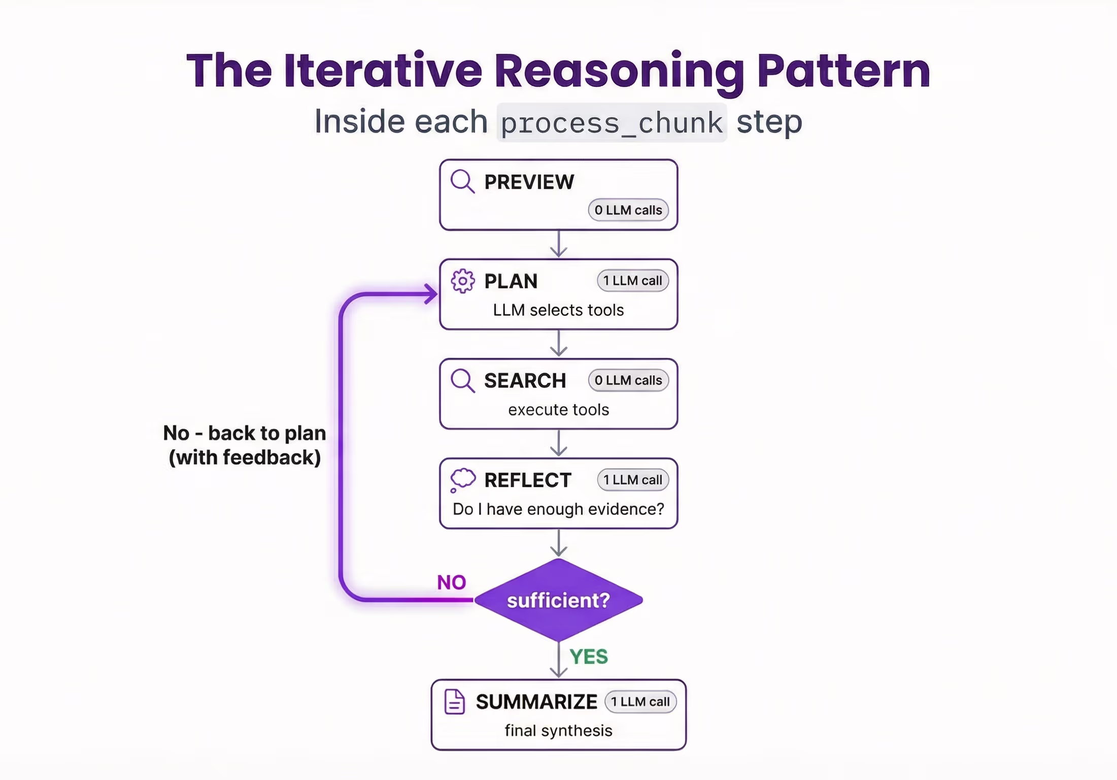
Each plan+reflect iteration costs 2 LLM calls. The final summarize costs 1. So max_iterations=6 allows up to 2 full search-reflect rounds plus the final synthesis.
One clarification on terminology: in the original RLM paper, “recursive” refers to symbolic recursion inside a REPL, where the model writes code that can programmatically invoke sub-model calls over slices or transformations of the input and store intermediate results as variables. A reflect step is a useful control mechanism for deciding whether to keep searching, but recursion in the RLM sense is about those programmatic sub-calls inside the environment, not reflection alone. In the code, this looks like:
while llm_calls < max_iterations - 1:  # Reserve 1 call for summarize
    # PLAN: LLM decides which tools to use
    plan_response = llm_call(SEARCH_PLAN_SYSTEM, plan_prompt, json_mode=True)
    llm_calls += 1

    # SEARCH: Execute the planned tools (no LLM calls)
    for search in searches:
        result = _execute_search(chunk_emails, search)

    # REFLECT: Is the evidence sufficient?
    reflect_response = llm_call(REFLECT_SYSTEM, reflect_prompt, json_mode=True)
    llm_calls += 1

    if sufficient:
        break  # Move to summarize
    # else: loop back with reflect_feedback guiding the next plan

# SUMMARIZE: Final synthesis
summary = llm_call(SUMMARIZE_SYSTEM, summarize_prompt, json_mode=True)
The 5 Typed Tools
Instead of giving the model a full REPL where it can write arbitrary Python, this implementation constrains it to 5 typed, deterministic tools:
TOOL_DESCRIPTIONS = {
    "grep":      "grep_emails(pattern) - Search email bodies/subjects by regex",
    "sender":    "filter_by_sender(sender) - Filter by sender name/email",
    "recipient": "filter_by_recipient(recipient) - Filter by recipient",
    "date":      "filter_by_date(start, end) - Filter by ISO date range",
    "count":     "count_matches(pattern) - Count regex matches across emails",
}
This is a deliberate design choice. The original RLM paper gives the model a full REPL, and DSPy’s dspy.RLM defaults to executing code in a local sandbox (Deno + Pyodide), and can be configured with different interpreters depending on your security and dependency requirements. In production, though, sandboxing alone doesn’t cover the whole story. You also want to constrain the agent’s action space so runs are auditable, deterministic where possible, and resistant to prompt injection and “excessive agency” style failures. This aligns with the OWASP LLM Top 10 categories: prompt injection (LLM01), insecure output handling (LLM02), model denial of service via runaway computation (LLM04), and excessive agency (LLM08).
We made this trade-off deliberately. In production, you want to know exactly what the model can do, not hope it writes safe code. You lose some generality but gain safety, auditability, and consistent trajectory events.
Two-Layer Budget Control
The pipeline enforces budgets at two levels:
# Pipeline-level: controls DAG width (how many chunks)
max_chunks = min(max(max_chunks, 1), 10)

# Step-level: controls LLM calls per chunk
max_iterations = min(max(max_iterations, 2), 12)
Neither layer alone is sufficient. Without pipeline-level control, the LLM could decide to create 1,000 chunks. Without step-level control, a single chunk could loop forever. Together, they put a hard ceiling on both the total parallelism and the per-chunk LLM spend.
This matters because of the heavy-tail cost profile mentioned earlier. You need to track p95 cost per chunk, not just averages.
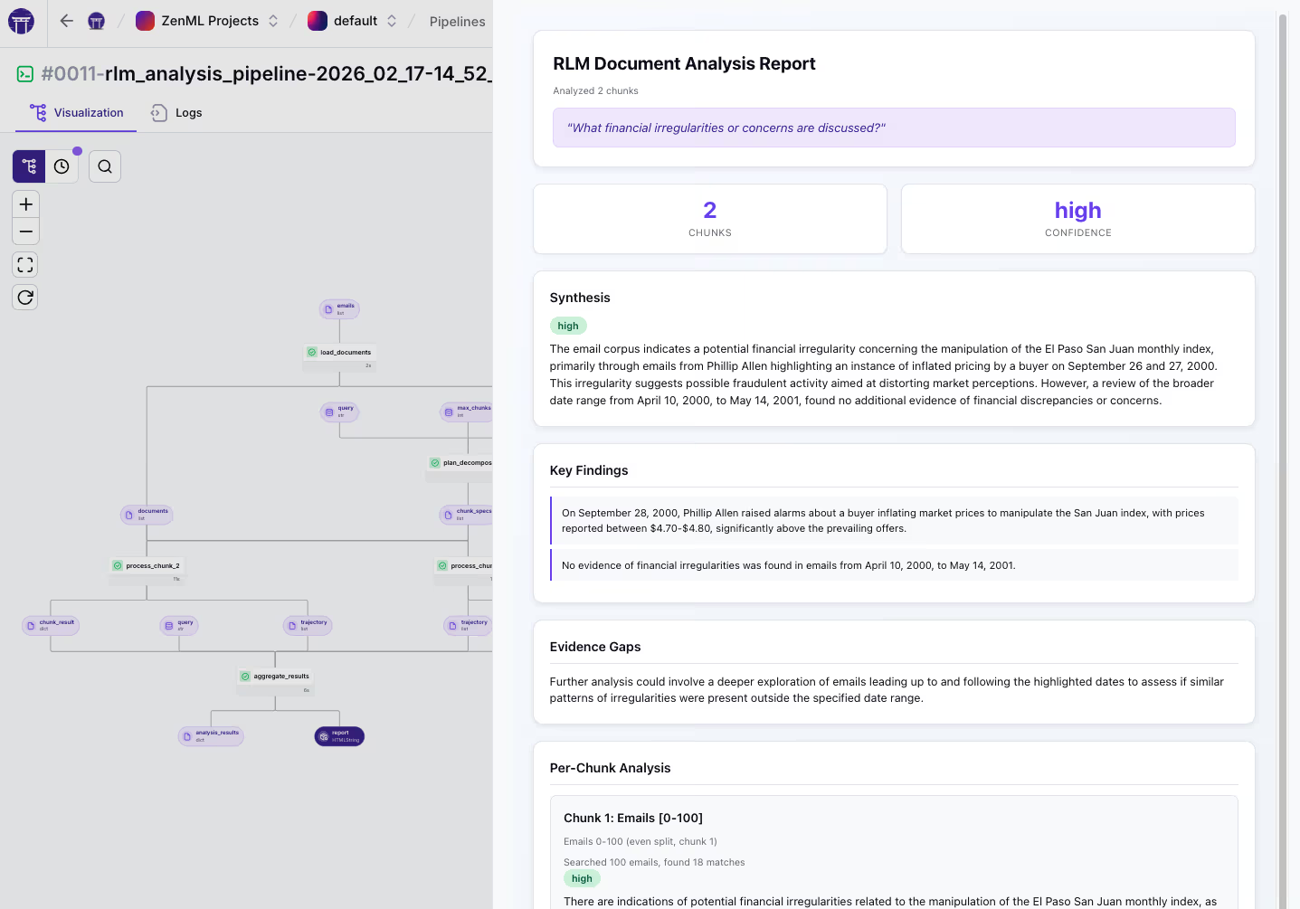
The Trajectory Artifact: Seeing What the Model Did
This is where it clicks for most people.
Every action in the RLM loop gets logged to a trajectory artifact. Here’s what one looks like, stored as a JSON artifact in ZenML:
[
  {"step": "preview", "action": "Examined 15 emails", "output": "Chunk contains 15 emails, Date range: 2001-01..."},
  {"step": "plan", "iteration": 1, "action": "Planned 3 searches", "searches": [{"tool": "grep", "reason": "Search for LJM references"}]},
  {"step": "search", "iteration": 1, "tool": "grep", "args": {"pattern": "LJM"}, "match_count": 7},
  {"step": "extract", "iteration": 1, "new_matches": 7, "total_matches": 7},
  {"step": "reflect", "iteration": 1, "sufficient": false, "reasoning": "Found LJM mentions but need dates to establish timeline..."},
  {"step": "plan", "iteration": 2, "action": "Planned 1 searches", "searches": [{"tool": "date", "reason": "Filter to early 2001"}]},
  {"step": "search", "iteration": 2, "tool": "date", "args": {"start": "2001-01-01", "end": "2001-06-30"}, "match_count": 4},
  {"step": "reflect", "iteration": 2, "sufficient": true, "reasoning": "Have enough evidence about LJM timeline"},
  {"step": "summarize", "finding_preview": "4 emails from early 2001 discuss LJM unwinding...", "confidence": "high", "total_iterations": 2, "total_llm_calls": 5}
]
This matters for three reasons:
Debugging. “Why did the model say X?” Click into the step, read the trajectory. You can see exactly which tools it called, what it found, and why it decided the evidence was sufficient (or not).
Cost attribution. Each trajectory event is tied to a step with logged metadata: duration, LLM calls, matches found. The log_metadata call at the end of each process_chunk records everything you need for per-chunk cost breakdown, without writing any custom logging.
log_metadata(
    metadata={
        "chunk_range": f"{start_idx}-{end_idx}",
        "chunk_size": len(chunk_emails),
        "llm_calls": llm_calls,
        "iterations": iteration,
        "matches_found": len(all_matches),
        "duration_s": duration,
    }
)
Reproducibility. Trajectory + artifacts = you can reconstruct exactly what happened in any chunk, months later. This is the same instinct behind good experiment tracking, applied to LLM reasoning.
A trajectory is basically a structured trace: a sequence of decisions, tool calls, and evidence. That framing is becoming standard. OpenTelemetry now defines GenAI semantic conventions for events and spans, including model name, token usage, and opt-in capture of inputs and outputs. Thinking of trajectories as traces makes it easier to plug RLM workloads into existing observability practices.
Try It Yourself
The full example is in the ZenML repo and runs locally with just an OpenAI API key:
git clone https://github.com/zenml-io/zenml.git
cd zenml/examples/rlm_document_analysis
pip install -r requirements.txt
export OPENAI_API_KEY="your-key"

# Run with the bundled sample data (60 synthetic Enron-style emails)
python run.py --query "What were the key financial irregularities?"

# Or scale up with the full Enron dataset from Hugging Face
pip install datasets
python setup_data.py
python run.py --source data/emails.json --max-chunks 8
The pipeline works without an API key too (it falls back to keyword matching), so you can explore the dynamic pipeline structure without spending anything.
A few things to note:
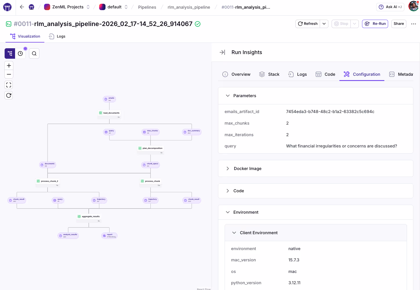
- The dynamic DAG is visible in the ZenML dashboard. Each
process_chunkis a separate step you can click into. - The example includes a deployable UI for running queries interactively.
- For Kubernetes deployment, it's a stack configuration change, not a code rewrite.
Practical notes: Dynamic pipelines are experimental and have orchestrator-specific support for isolated parallel steps. Also, .load() is synchronous: use it for control flow, but avoid loading large artifacts unnecessarily. Parallel logging can be noisy today because logs from concurrent steps may interleave.
Links:
- The example code
- ZenML dynamic pipelines documentation
- The RLM paper (Zhang, Kraska, Khattab)
- DSPy RLM module
What’s Next
There are several natural extensions we’re excited about:
Deeper recursion. The current example is depth-1: decompose, process chunks, aggregate. Depth-2+ would have process_chunk spawn sub-pipelines for really large corpora. ZenML dynamic pipelines don’t yet support the spawning of sub-pipelines, but we kept it simple for the initial example.
Evaluation pipeline. Run the same queries through vanilla LLM, RAG, and the RLM pipeline, then compare accuracy, cost, and latency. This is a natural follow-up task.
dspy.RLM inside steps. You can drop dspy.RLM directly into the process_chunk step as the reasoning engine while keeping ZenML as the orchestration layer. The trajectory output plugs right in. DSPy builds the LLM programs. ZenML runs them in production.
Community contributions welcome. If you extend this for your own use case, we’d love to hear about it. The example is on GitHub and the pipeline structure is designed to be adapted.